Causality in Machine Learning? Is That a Thing?
February 24, 2020

Kade Young, PhD Candidate
February 24, 2020
Kade Young, PhD Candidate
Causality. That’s the gold standard for all investigative statisticians. Investigative, meaning I give you data corresponding with a certain outcome, and you find what causes the outcome. It is somewhat simpler to find correlation, but that is entirely different than causality. For example, the number of firefighters sent to a fire directly correlates to the amount of damage a fire does. Now, does that mean firefighters actually cause more damage? Absolutely not. It is known that smoking is highly correlated with lung cancer, but it is immensely more powerful to state that smoking causes cancer.
So, why do some modern statistical practices seem to care little about extracting causality? For example, neural networks, a very popular machine learning technique at the moment, is notorious for sacrificing interpretability to improve accuracy. The science part of data science, however, is the investigation of these causal relationships.
I recently had the opportunity to experience this first hand while working on an industry research project. The project involves rather large data, almost 2 million observations with around 400 covariates with the end goal of binary classification. The unique issue is that these covariates can be grouped into roughly 10 categories and the industry wanted insight into which of these categories of features were most responsible for the value our model predicted. So how do we go about backing out this insight from machine learning techniques?
Take our example of a neural network; within these frameworks there are a variety of mid-layer techniques that have been developed to introduce flexibility, such as convolutional layers and bias nodes. However, this flexibility comes at a price. These mid-layer methods introduce weights and/or feature mappings that essentially eliminate the possibility of interpretable mid-layer output. In fact, convolutional layers by design map a region of inputs to a single node in the next layer, thereby obfuscating the feature category or categories that are driving decision making. However, if we focus solely on feed-forward networks without allowing each category to inter-mingle with others (i.e. not allowing the network to be fully connected between categories), we might be able to backtrack and use mid-layer output as a measure of categorical importance. With this in mind, there are certain network architectures that can be applied to give these insights into the importance of each category.
So, what if we know each category’s “importance”? How does that help us change the outcome? This turns into a decision boundary problem. Imagine the space of covariates. In our specific case, it is around 400 dimensions, but, to simplify, imagine a 2-dimensional space. The decision boundary in the 2-dimension case is essentially a line dividing the 2-dimensional plane; every data point on one side of the boundary is classified as one outcome, every point on the other side is classified as the other outcome. Now, in 400 dimensions, this is not easy to visualize, but, if we can find which specific covariates we can change slightly in order to change classification (i.e. get to the decision boundary), we can get some rudimentary idea of where sensitivity in outcome change can happen.
It is important to note that bridging this concept to actual causality requires much more work, but it seems to be a good start. As always here at Laber Labs, there is a lot of work to be done to flesh this out. However, this remains an intriguing and ever-expanding subset of machine learning.
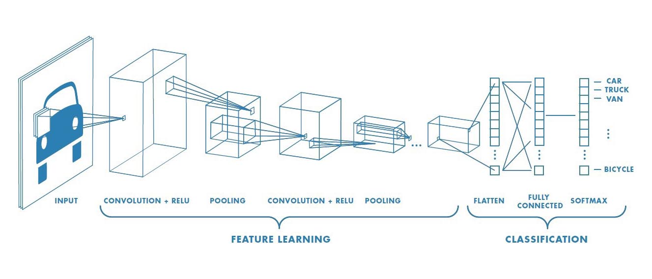
Source: "A Comprehensive Guide to Convolutional Neural Networks - the ELI5 way" by Sumit Saha
Kade is a PhD Candidate whose research interests lie in sports analytics, computer vision, and reinforcement learning. His current research focuses on reinforcement learning in personalized medicine/education and object detection in sports. We asked a fellow Laber Labs colleague to ask Kade a probing question
Explain why American football is a more intellectual endeavor than statistics to a Frenchman who specializes in the liberal arts.
The modern statistician has the luxury of time; time to think about the problems they are faced with. How do I design this trial? How do I estimate an optimal treatment? Football players on the other hand, do not have time. An average of 25 seconds elapse between successive plays. This time is used to diagnose tendencies, think of what play your team is running, think of what your opponent might do, get in the right position, and focus your eyes on the right things to be successful in the following play. The higher the level of football being played, requires more of these decisions to be made and faster. This does not mention that the penalty for making a wrong decision is more than likely bodily harm. This process happens anywhere from 60 to 120 times in a single game, so mental and physical fatigue undoubtedly will set in.